Type S Thermocouple Calibration
For those using Mosaic's Thermocouple Wildcard, thermocouple voltages are automatically converted to temperatures with high accuracy by the included software drivers.
For those not using the Thermocouple Wildcard, but still looking for accurate conversion equations for thermocouple measurement, here are some calibration functions and coefficients that should be helpful.
Conversion equations for cold junction temperature-to-voltage and measurement voltage-to-temperature are often based on high-order polynomials. For example, the National Institute of Standards and Technology ITS-90 database of thermocouple values provides a high order polynomial formula with coefficients curve fitted to type S thermocouple data.
Unfortunately, even high order polynomials are often not too accurate – they exhibit systematic errors as the polynomials oscillate around the actual data, as shown in these curve fits to Type K thermocouples.
There is a better way – using rational polynomial functions. On this page we show you how to convert type S thermocouple voltage to temperature using rational polynomial functions more accurately and efficiently than you could using the more common high order polynomials.
Rational polynomial fits produce an order of magnitude lower errors than the type S NIST ITS-90 thermocouple coefficients for direct (measurement) and inverse (cold junction compensation) polynomials.
Type S calibration equation
A curve fitted rational polynomial function for Type S thermocouples is used for computing temperature from measured thermocouple voltage. The calibration equation uses a ratio of two smaller order polynomials rather than one large order polynomial. Using a least squares curve fitting we fit the National Institute of Standards and Technology (NIST) ITS-90 type S thermocouple data with a rational function of this form:
where T is the thermocouple temperature (in °C), V is the thermocouple voltage (in millivolts), and To, Vo, and the pi and qi are coefficients. The function uses a ratio of two polynomials, P/Q, in this case a fourth order to a third order polynomial. The second form of the equation emphasizes the most efficient order of operations.
The coefficients, To, Vo, pi and qi were found by performing a least squares curve fit to the NIST data for type S thermocouples. The full temperature range is broken into several sub-ranges, and a different set of coefficients used for each. The coefficients, fitted data and charts of residual errors may be found in this Excel spreadsheet of thermocouple data.
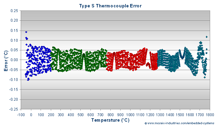
The following table contains calibration coefficients for Type S thermocouple wire. The graph shows residual errors after calibrating the thermocouple with a rational function of polynomials. Most of the residual error results from rounding of the NIST provided voltage values to the nearest microvolt. The rational function approximation interpolates the data well so that computed values of temperature are more accurate than the residuals plots would indicate.
The following table provides the rational polynomial calibration coefficients for Type S thermocouple wires.
| Range | ||||
|---|---|---|---|---|
| Voltage: | -0.236 to 1.441 mV | 1.441 to 6.913 mV | 6.913 to 12.856 mV | 12.856 to 18.693 mV |
| Temperature: | -50 to 200°C | 200 to 760°C | 760 to 1275°C | 1275 to 1768°C |
| Coefficients | ||||
| T0 | 1.3792630E+02 | 4.7673468E+02 | 9.7946589E+02 | 1.6010461E+03 |
| V0 | 9.3395024E-01 | 4.0037367E+00 | 9.3508283E+00 | 1.6789315E+01 |
| p1 | 1.2761836E+02 | 1.0174512E+02 | 8.7126730E+01 | 8.4315871E+01 |
| p2 | 1.1089050E+02 | -8.9306371E+00 | -2.3139202E+00 | -1.0185043E+01 |
| p3 | 1.9898457E+01 | -4.2942435E+00 | -3.2682118E-02 | -4.6283954E+00 |
| p4 | 9.6152996E-02 | 2.0453847E-01 | 4.6090022E-03 | -1.0158749E+00 |
| q1 | 9.6545918E-01 | -7.1227776E-02 | -1.4299790E-02 | -1.2877783E-01 |
| q2 | 2.0813850E-01 | -4.4618306E-02 | -1.2289882E-03 | -5.5802216E-02 |
| q3 | 0.0 | 1.6822887E-03 | 0.0 | -1.2146518E-02 |
Type S thermocouple accuracy and calibration error
This graph shows the residual errors that remain after calibration with the above coefficients:
Most of the residual error in the above graph results from rounding of the NIST provided voltage values to the nearest microvolt. You can see the rounding errors as aliasing or Moiré patterns in the data.
The rational function approximation interpolates the type S data well so that computed values of temperature are more accurate than the residuals plots would indicate.
Computing type S cold junction voltages
Your type S thermocouple may be terminated at a cold junction temperature other than 0°C. If so, you must measure the temperature of the cold junction using another sensor, perhaps a thermistor. You can then compute a cold junction voltage from that measured temperature, and use it to compensate the type S thermocouple voltage before converting the thermocouple voltage to a temperature.
In that case you need the inverse transform, that is, an equation for converting temperature into voltage. You don't need a valid equation for a wide temperature range as the cold junction is likely to be placed at ambient temperature. Usually a range of -20 to +70°C is sufficient.
To convert temperature to voltage, you can again use a rational function approximation of the form,
where TCJ is the cold junction temperature, VCJ is the computed cold junction voltage, and the T0, V0, pi and qi are coefficients.
To learn more about cold junction compensation you can consult How To Do Cold Junction Compensation, and you can find the coefficients here:


